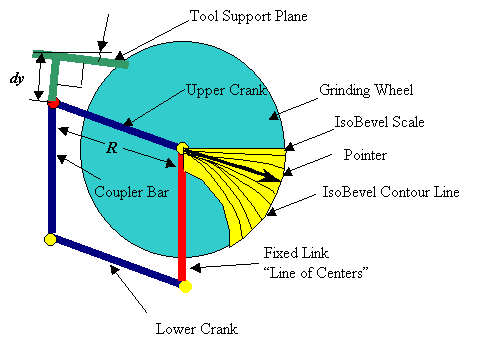
IsoBevel curves are a graphical representation of the level curves or contour lines of a function of two variables. These two variables are the grinding wheel radius and the angular position of the cranks of the parallelogram linkage. The attitude of the toolrest plane is fixed with respect to the ground plane by being rigidly connected to the coupler bar of the parallelogram linkage. In the derivation that follows we will assume without loss of generality that the toolrest plane is parallel to the ground plane for all crank angles. Inclined toolrest planes may be accommodated by rotating the scale by the toolrest inclination angle.
The following derivation makes use of vector and scalar
quantities. Vectors quantities are
denoted by bold characters while scalars are italicized.
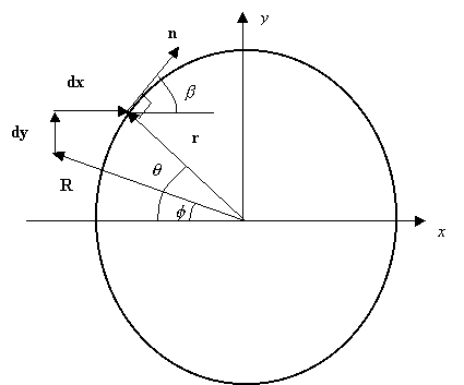
Consider a grinding wheel of radius r and a crank arm with a pivot at the grinding wheel center and the other at radius R. A horizontal plane is situated a distance dy above the right pivot pin of the crank arm.
Inclination Angle

Idealized model
 |
The x axis is parallel to the ground plane.
The blade centerline is denoted by the vector
![]() and will be ground to a bevel angle
and will be ground to a bevel angle
![]() when presented to the grinding
wheel. The angle
when presented to the grinding
wheel. The angle
![]() specifies the angular position of the point of contact between the toolrest
plane and grinding wheel. The angle
specifies the angular position of the point of contact between the toolrest
plane and grinding wheel. The angle
![]() defines the angular position of the
crank. Since the toolrest plane
intersects the grinding wheel periphery at r, we must find a vector that
is perpendicular to r. This
vector will be denoted as n and it will be a unit vector
(magnitude = 1). Since r and
n are normal, the vector dot product
defines the angular position of the
crank. Since the toolrest plane
intersects the grinding wheel periphery at r, we must find a vector that
is perpendicular to r. This
vector will be denoted as n and it will be a unit vector
(magnitude = 1). Since r and
n are normal, the vector dot product
![]() . Breaking r and n into component form and taking the dot product
we obtain:
. Breaking r and n into component form and taking the dot product
we obtain:
![]()
thus:
![]()
and it follows that:
![]()
Our objective is to determine
![]() as a function of the measurable variables r and
as a function of the measurable variables r and
![]() . We know that the vector sum of R,dy
and dx is equal to the
radius vector r, thus:
. We know that the vector sum of R,dy
and dx is equal to the
radius vector r, thus:
![]()
or in component form:
![]()
setting the
![]() components equal to one another we
find:
components equal to one another we
find:
![]()
substituting
![]() for
for
![]() we obtain:
we obtain:
![]()
solving for
![]() we obtain the desired relationship:
we obtain the desired relationship:
![]() (1)
(1)
or alternatively in Cartesian coordinates:
 (2)
(2)
which is a convenient form for computer implementation.
These expressions are remarkably simple when compared to the more complex
equivalent expression given in the patent.
The expression in the patent was derived using geometric and
trigonometric (law of sines and cosines) principles while the expressions shown
here were derived using a more elegant vector based approach.
 |
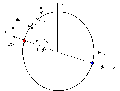
We now have expressions that will generate a value for the
bevel angle
![]() at the point colored in red.
This point corresponds to a point on the centerline of the upper crank at
a distance r from the center. Since
the upper crank would obscure this point we must determine the value of the
bevel angle
at the point colored in red.
This point corresponds to a point on the centerline of the upper crank at
a distance r from the center. Since
the upper crank would obscure this point we must determine the value of the
bevel angle
![]() at some point that is not obscured by any part of the mechanism so we simply
choose the point colored in blue that is 180 degrees from the red point at a
distance r measured from the center.
To calculate the bevel angle at this point we simply calculate
at some point that is not obscured by any part of the mechanism so we simply
choose the point colored in blue that is 180 degrees from the red point at a
distance r measured from the center.
To calculate the bevel angle at this point we simply calculate
![]() . By plotting the lines of constant
bevel angle at (-x,-y) we can generate an IsoBevel scale that indicates
the bevel angle that will be obtained for a particular grinding wheel radius and
linkage position. A pointer of
length r that passes through (0,0) and the blue point will intersect one
of the IsoBevel curves and will convey to the user the bevel angle that will be
obtained for grinding wheels and linkages of arbitrary size.
. By plotting the lines of constant
bevel angle at (-x,-y) we can generate an IsoBevel scale that indicates
the bevel angle that will be obtained for a particular grinding wheel radius and
linkage position. A pointer of
length r that passes through (0,0) and the blue point will intersect one
of the IsoBevel curves and will convey to the user the bevel angle that will be
obtained for grinding wheels and linkages of arbitrary size.
Expression 2 is in a convenient form for computer
implementation because we are interested in locating the points on the IsoBevel
curves in Cartesian (x,y) coordinates so that a CAD package can read them. The
simplest approach to generating IsoBevel curves involves generating an unsorted
set of bevel angles over a large number of points (x,y) in the domain of
interest. Gridding software can then be used to estimate the bevel angles at
specific points on a grid and connect points of equal value.
Gridding and contouring software is widely used in engineering, mapping
and weather prediction and is quite sophisticated and can handle randomly spaced
data. In our case, we have a well
defined function on (x,y) and we can use this to our advantage and sidestep the
complicated gridding and contouring process.
The idea is simple. To find
points on the IsoBevel curves we fix
![]() and calculate y for a range
of x . In other words
we must find
and calculate y for a range
of x . In other words
we must find
![]() . It turns out that when solving
. It turns out that when solving
![]() for y four possible answers
can result (there are four roots to this equation).
Fortunately, in most cases we are only interested in one of these roots
because we will only be generating curves over a limited range of (x,y).
Closed form analytic expressions for
for y four possible answers
can result (there are four roots to this equation).
Fortunately, in most cases we are only interested in one of these roots
because we will only be generating curves over a limited range of (x,y).
Closed form analytic expressions for
![]() are quite complicated and we
therefore resort to an iterative numerical method.
Any number of root finding techniques can be used (e.g. Golden Section,
Newton’s method, Regula Falsi etc.). In
this case I chose to use a Fixed-Point Iteration.
To use this approach we simply manipulate Equation 2 so that y
appears on the left-hand side of the equation.
are quite complicated and we
therefore resort to an iterative numerical method.
Any number of root finding techniques can be used (e.g. Golden Section,
Newton’s method, Regula Falsi etc.). In
this case I chose to use a Fixed-Point Iteration.
To use this approach we simply manipulate Equation 2 so that y
appears on the left-hand side of the equation.
![]() (3)
(3)
We now apply the subscript k to the y’s on the right hand side to denote the past estimate of y. The k+1 subscript denotes the updated (more accurate) estimate of y that satisfies Equation (2).
 (4)
(4)
Equation 4 is the fixed point iteration that defines a
sequence of estimates for y that will approach to the true value of y
that satisfies Equation (2). The
initial or starting value
![]() is somewhat arbitrarily set equal
to 1 (0 may be a better starting point since all curves intersect at (0,0)).
In practice the sequences converge quite rapidly and iteration is
terminated when:
is somewhat arbitrarily set equal
to 1 (0 may be a better starting point since all curves intersect at (0,0)).
In practice the sequences converge quite rapidly and iteration is
terminated when:
![]()
This condition indicates that further iterations will not
result in a significant improvement in accuracy.
This technique works quite well; however, the only pitfall
encountered to date is the possibility of specifying linkage geometries that
require the computation of two roots due to the curve taking on two values of
y for a given x. This
will result in the affected curves being truncated when the slope of the
IsoBevel curve goes to infinity (i.e. vertical line).
The problem can be solved by providing a new initial value for
![]() that is closer to the second root;
however, this feature has not been implemented since you can always specify a
linkage geometry that eliminates this problem.
that is closer to the second root;
however, this feature has not been implemented since you can always specify a
linkage geometry that eliminates this problem.
IsoBevel™ Home
Building an IsoBevel Grinder/Sharpener
IsoBevel Scale Generation: Software Manual
Copyright © 2000, David B. Doman, PhD, All rights reserved.